Exploring a Convolutional Neural Network for classifying handwritten digits
This post was exported directly from a Jupyter notebook (using the nbconvert utility which is built into Jupyter), demonstrating another way of writing posts.
In this post, we explore using convolutional neural networks implemented in Tensorflow for classifying the handwritten digits in the MNIST dataset. We design and train a relatively simple network with approximately 19,000 weights which is still able to classify the dataset with approximately 99% accuracy. Being quite simple, we are able to take a closer look at the internals of the network to see what it learns and how the classification process works.
import pandas as pd
import seaborn as sns
import matplotlib.pyplot as plt
import numpy as np
import tensorflow as tf
from tensorflow import keras
Data preprocessing
Load in the data from the CSV files in the data directory. These file contain one image per row. The training dataset has labels, while the testing dataset does not. For this reason, we are only interested here in using the training data to experiment with, so that we can check how we are doing.
train = pd.read_csv('data/train.csv')
test = pd.read_csv('data/test.csv')

print(f'The dataset contains {train.shape} training images ' \
        f'and {test.shape} testing images')
The dataset contains (42000, 785) training images and (28000, 784) testing images
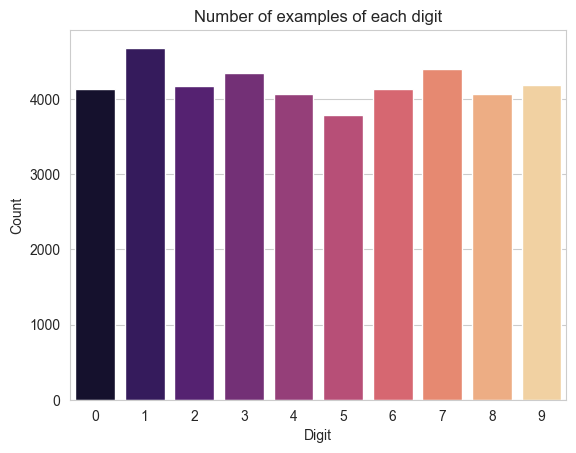
Visualise the number of images we have for each digit. Generally, they are pretty evenly distributed.
sns.countplot(x=train.label, palette='magma')
plt.xlabel('Digit')
plt.ylabel('Count')
plt.title('Number of examples of each digit')
plt.show()
Preprocess the images by splitting the labels out into a separate array, and converting the row vector respresenting each digit into a more traditional matrix of pixel values. This matrix has an extra dimension to signify to Tensorflow that there is only a single colour channel. For convenience, we also create a digit_images array, which splits the images up into groups of images corresponding to different digits, so we can easily extract examples corresponding to a given digit.
labels = train.label
images = np.array(train.drop(columns=['label'])) / 255.0
test_images = np.array(test)

print('Initially, the images array has each image as a row, with shape', images.shape)
images = images.reshape(-1, 28, 28, 1)
test_images = test_images.reshape(-1, 28, 28, 1)
print('After reshaping, the images array has shape', images.shape)

digit_images = []
for i in range(10):
    digit_images.append(images[labels == i, :, :, :])
Initially, the images array has each image as a row, with shape (42000, 784)
After reshaping, the images array has shape (42000, 28, 28, 1)
We can visualise the training images by plotting an example of each digit.
fig, axes = plt.subplots(nrows=1, ncols=10, figsize=(15, 5))
for i in range(10):
    axes[i].imshow(digit_images[i][0], cmap='gray')
    axes[i].set_title(f'{i}')
    axes[i].axis('off')
plt.show()

Now we can use sklearn to divide our data into a training set and a validation set. We select 80% of the data to be the training set, corresponding to 33,600 images.
from sklearn.model_selection import train_test_split

X_train, X_val, y_train, y_val = train_test_split(
    images, labels,
    test_size=0.2,
    random_state=2
)
For full compatibility with Tensorflow, we set up Datsets for our training and validation images from the step above. To ensure our data throughput performs well, we use batching, caching and prefetching on the datasets. We also shuffle the training set so that they will be seen in a different order in each training epoch to avoid stagnation. Finally, we repeat the training set to make full use of the augmentation steps we are going to apply later.
AUTOTUNE = tf.data.AUTOTUNE
BATCH_SIZE = 256
SHUFFLE_BUFFER = 5
N_REPEATS = 3

train_dataset = (
    tf.data.Dataset.from_tensor_slices((X_train, y_train))
    .batch(BATCH_SIZE)
    .cache()
    .prefetch(buffer_size=AUTOTUNE)
    .shuffle(buffer_size=SHUFFLE_BUFFER)
    .repeat(N_REPEATS)
)

validation_dataset = (
    tf.data.Dataset.from_tensor_slices((X_val, y_val))
    .batch(BATCH_SIZE)
    .cache()
    .prefetch(buffer_size=AUTOTUNE)
)
Network definition
Now we define the architecture of the convolutional neural network we will be using. We split up the definition of the network into separate chunks which will allow us to interrogate its behaviour post-training more easily. Broadly speaking, the structure is composed of three parts.
Preprocessing layers
We use the RandomRotation and RandomTranslation layers to augment the dataset to include examples seen from slightly different angles and centered differently. This is followed by a Normalization step where we ensure that each pixel value is scaled to have mean 0 and variance 1. The normalisation helps ensure we are biased into the sensitive regime of the network.
Convolutional layers
Next, the image is passed through a sequence of convolutional layers.
- First, a set of 5x5 kernels producing
n_convolution_filtersfeature maps, - Second, a
MaxPool2dlayer to collapse the output of the layer above, - Third, a set of 5x5 kernels producing
2 * n_convolution_filtersfeature maps, - Fourth, a set of 3x3 kernels producing
3 * n_convolution_filtersfeature maps, - Finally, the output from the feature maps is put through a
GlobalAveragePoolinglayer to produce a ‘barcode’ for each image.
In all of these convolutional layers, we use a leaky_relu activation function to ensure there is some sensitivity to inputs smaller than 0, and couple this with some $\ell^2$ regularisation.
Dense head
The barcodes output by the convolutional layers are then interpreted and classified by the final dense layers, which output the predicted class in 1-hot encoded form.
from keras import Sequential
from keras import layers
from keras import activations

history = {}

n_convolution_filters = 20
regulariser = tf.keras.regularizers.L2(l2=0.0001)

# Definition of a 'leaky' version of relu, which
# retains some gradient for inputs x < 0
def leaky_relu(x):
    return activations.relu(x, alpha=0.01)

# Preprocessing layers
preprocessing_layers = Sequential([
    layers.Normalization(input_shape=[28, 28, 1]),
])

# Convolutional feature map extractors
conv_layers = [
    # First convolution and pooling block
    Sequential([
        layers.Conv2D(
            filters=n_convolution_filters,
            kernel_size=5, padding='valid',
            activation=leaky_relu,
            kernel_regularizer=regulariser
        ),
        layers.MaxPool2D(pool_size=2),
    ]),

    # Second convolution block
    Sequential([
        layers.Conv2D(
            filters=1*n_convolution_filters,
            kernel_size=5, padding='valid',
            activation=leaky_relu,
            kernel_regularizer=regulariser
        ),
    ]),

    # Third convolution block
    Sequential([
        layers.Conv2D(
            filters=2*n_convolution_filters,
            kernel_size=3, padding='valid',
            activation=leaky_relu,
            kernel_regularizer=regulariser
        ),
    ])
]

model = Sequential([
    # Preprocessing layers
    layers.RandomRotation(factor=0.1, fill_mode='constant', input_shape=[28, 28, 1]),
    layers.RandomTranslation(height_factor=0.1, width_factor=0.1),

    preprocessing_layers,

    # Convolutional feature map extractors
    conv_layers[0],
    conv_layers[1],
    conv_layers[2],

    # Pooling: summarise each channel into a single feature
    layers.GlobalAveragePooling2D(),

    # Dense classifier head
    layers.Flatten(),
    layers.Dense(units=20, activation=leaky_relu),
    layers.Dense(units=10, activation='softmax')
])

# Compile the model with an optimiser
model.compile(
    optimizer = tf.keras.optimizers.Adam(epsilon=0.0001),
    loss = 'sparse_categorical_crossentropy',
    metrics = ['accuracy', 'sparse_categorical_accuracy']
)

model.summary()
Model: "sequential_4"
_________________________________________________________________
 Layer (type)                Output Shape              Param #
=================================================================
 random_rotation (RandomRota  (None, 28, 28, 1)        0
 tion)

 random_translation (RandomT  (None, 28, 28, 1)        0
 ranslation)

 sequential (Sequential)     (None, 28, 28, 1)         3

 sequential_1 (Sequential)   (None, 12, 12, 20)        520

 sequential_2 (Sequential)   (None, 8, 8, 20)          10020

 sequential_3 (Sequential)   (None, 6, 6, 40)          7240

 global_average_pooling2d (G  (None, 40)               0
 lobalAveragePooling2D)

 flatten (Flatten)           (None, 40)                0

 dense (Dense)               (None, 20)                820

 dense_1 (Dense)             (None, 10)                210

=================================================================
Total params: 18,813
Trainable params: 18,810
Non-trainable params: 3
_________________________________________________________________
Network training
The network is trained in the usual way for some set number of epochs, and the resulting loss curves are appended to the history object. This enables us to incrementally train the model yet retain the complete history of the metrics.
latest_history = model.fit(
    train_dataset,
    validation_data=validation_dataset,
    epochs=80,
    verbose=1
)

latest_history = latest_history.history
for k in latest_history.keys():
    if k in history.keys():
        history[k] = np.concatenate((history[k], latest_history[k]))
    else:
        history[k] = latest_history[k]
Epoch 1/80
396/396 [==============================] - 8s 9ms/step - loss: 1.3725 - accuracy: 0.5225 - sparse_categorical_accuracy: 0.5225 - val_loss: 0.4404 - val_accuracy: 0.8821 - val_sparse_categorical_accuracy: 0.8821
Epoch 2/80
396/396 [==============================] - 3s 8ms/step - loss: 0.6091 - accuracy: 0.8139 - sparse_categorical_accuracy: 0.8139 - val_loss: 0.2941 - val_accuracy: 0.9207 - val_sparse_categorical_accuracy: 0.9207

(...)

Epoch 79/80
396/396 [==============================] - 3s 8ms/step - loss: 0.0562 - accuracy: 0.9899 - sparse_categorical_accuracy: 0.9899 - val_loss: 0.0544 - val_accuracy: 0.9905 - val_sparse_categorical_accuracy: 0.9905
Epoch 80/80
396/396 [==============================] - 3s 8ms/step - loss: 0.0563 - accuracy: 0.9895 - sparse_categorical_accuracy: 0.9895 - val_loss: 0.0593 - val_accuracy: 0.9889 - val_sparse_categorical_accuracy: 0.9889
Post-training analysis
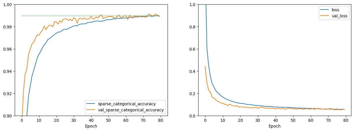
Plot the loss and metric curves to verify that the training process has converged appropriately
n_epochs = len(history['sparse_categorical_accuracy'])
last_accuracy = history['sparse_categorical_accuracy'][-1]

fig, axes = plt.subplots(nrows=1, ncols=2, figsize=(15, 5))

axes[0].plot(history['sparse_categorical_accuracy'], label='sparse_categorical_accuracy')
axes[0].plot(history['val_sparse_categorical_accuracy'], label='val_sparse_categorical_accuracy')
axes[0].plot([0, n_epochs], [last_accuracy, last_accuracy], ':')
axes[0].set_xlabel('Epoch')
axes[0].legend(loc='lower right')
axes[0].set_ylim(bottom=0.9, top=1.0)

axes[1].plot(history['loss'], label='loss')
axes[1].plot(history['val_loss'], label='val_loss')
axes[1].set_xlabel('Epoch')
axes[1].legend(loc='upper right')
axes[1].set_ylim(bottom=0.0, top=1.0)
plt.show()

model.evaluate(validation_dataset, verbose=2);
33/33 - 0s - loss: 0.0593 - accuracy: 0.9889 - sparse_categorical_accuracy: 0.9889 - 140ms/epoch - 4ms/step
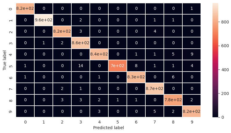
Assess the confusion matrix for the model, to determine whether there are any obvious problems.
import numpy as np
from sklearn.metrics import confusion_matrix
y_pred = model.predict(validation_dataset)
y_pred_class = np.argmax(y_pred, axis=1)
y_true = y_val

conf_mat = confusion_matrix(y_true, y_pred_class)

f, ax = plt.subplots(figsize=(10, 5))
sns.heatmap(conf_mat, annot=True, linewidths=0.01)
plt.xlabel('Predicted label')
plt.ylabel('True label')
sns.reset_orig()
Examining the trained network
Now we wish to look at the internals of the network, to understand what its convolutional kernels look like and what the output barcodes are like. For this, we first define some useful functions for extracting and plotting kernels, and for plotting the features maps produced by passing an input image through the kernels up to some specified bank. Note that we do not plot all of the kernels for the second and third banks of convolutional layers as there are simply too many.
n_preprocessing_layers = 2
n_filters_per_row = 10
n_rows = n_convolution_filters // n_filters_per_row

def show_filters(bank):
    fig, axes = plt.subplots(
        nrows=n_rows, ncols=n_filters_per_row,
        figsize=(3 * n_filters_per_row, 3 * n_rows + 2)
    )

    layer = conv_layers[bank].layers[0]
    weights = layer.weights[0].numpy()

    vmax = weights.max()
    vmin = weights.min()

    for j in range(n_rows):
        for i in range(n_filters_per_row):
            axes[j, i].imshow(
                weights[:, :, 0, i + j * n_filters_per_row],
                vmax=vmax, vmin=vmin
            )
            axes[j, i].set_title(i + j * n_filters_per_row)
    plt.show()

def show_feature_maps(image, bank):
    n_filters_in_bank = conv_layers[bank].weights[0].shape[-1]
    n_rows = n_filters_in_bank // n_filters_per_row

    fig, axes = plt.subplots(
        nrows=n_rows, ncols=n_filters_per_row,
        figsize=(3 * n_filters_per_row, 3 * n_rows + 2)
    )

    image = tf.convert_to_tensor([image])

    processed = preprocessing_layers.call(image)

    for b in range(bank + 1):
        processed = conv_layers[b].call(processed)

    vmax = processed.numpy().max()
    vmin = processed.numpy().min()

    for j in range(n_rows):
        for i in range(n_filters_per_row):
            axes[j, i].imshow(
                processed[0, :, :, i + j * n_filters_per_row],
                vmin=vmin, vmax=vmax
            )
            axes[j, i].set_title(i + j * n_filters_per_row)
    plt.show()
These are the filters in the first convolutional layer. As we can see, the network seems to have learnt to produce edge filters in various directions, amongst other patterns. There also seems to be some redundancy among the filters, implying that we may be able to get away with fewer feature maps (and thus fewer weights to train).
show_filters(0)

This is what a handwritten 0 looks like when passed through the first convolutional layer. We can see the different edge filters doing their job.
show_feature_maps(digit_images[0][0], 0)

Similarly, we can look at the effect on a handwritten 1. Horizontal edge features are largely zero for this.
show_feature_maps(digit_images[1][1], 0)

These are the feature maps produced by the third convolutional layer for an input of a 0.
show_feature_maps(digit_images[0][0], 2)
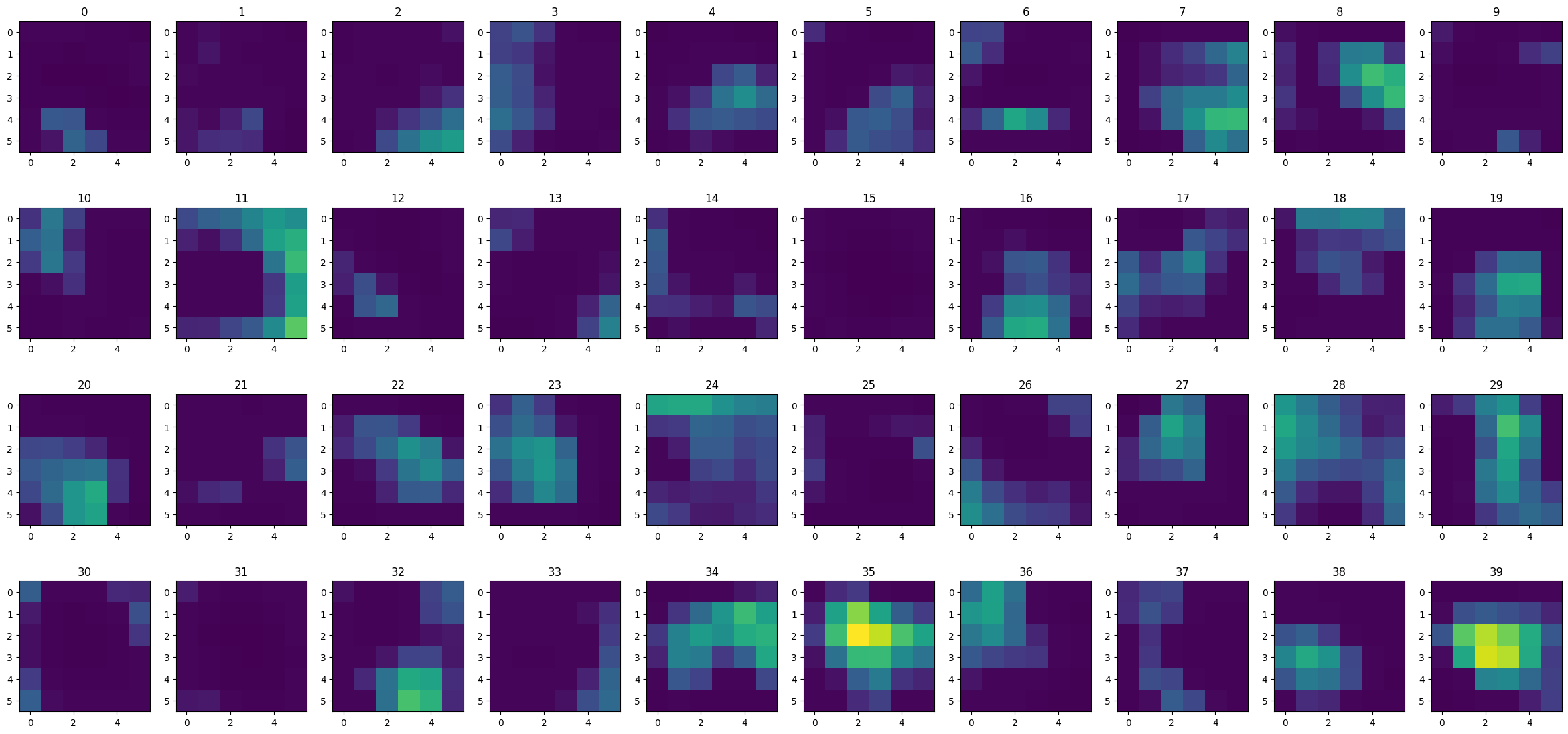
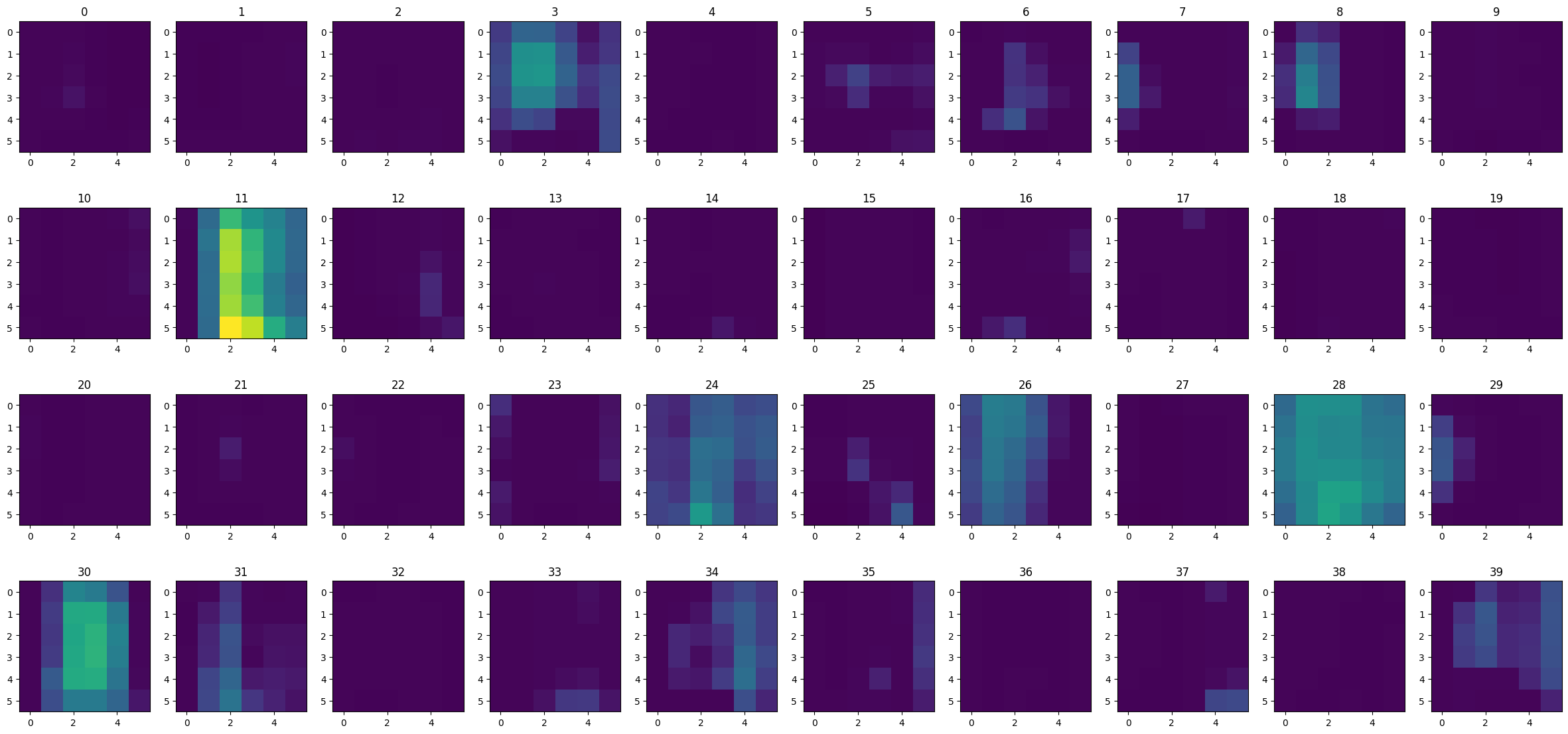
Here is the output from the third convolutional layer for an input of a 1. We can see that the big activations are in different places from those above. This indicates that the network has manged to separate the digits, and is what is used by the dense head layers to distinguish different digits.
show_feature_maps(digit_images[1][1], 2)
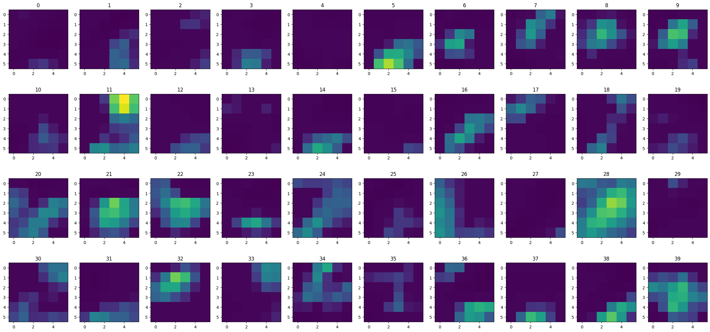
Here is the output from the third layer for a digit 2. Again, the key activations are in different places, and we are able to get a sense of which macroscopic features of a 2 some of the filters are looking for.
show_feature_maps(digit_images[2][1], 2)
The final step of the convolutional layers is to collapse the features maps down to a ‘barcode’, producing a single summary value for each feature map, using the GlobalAveragePooling layer. We introduce a some helper functions below to compute the barcode and plot it.
n_convolution_banks = 3

def barcode(image):
    image = tf.convert_to_tensor([image])
    processed = preprocessing_layers.call(image)
    for b in range(n_convolution_banks):
        processed = conv_layers[b].call(processed)
    return processed.numpy().mean(axis=(1, 2))

def show_barcode(barcode, axis):
    axis.imshow(barcode, cmap='gray')
    axis.axis('on')
    axis.get_xaxis().set_ticks([])
    axis.get_yaxis().set_ticks([])
First of all, we compute an average barcode over a subset of the data, which we will use to highlight common activations and enable us to de-trend the results below for easier visualisation. We see that there are some feature maps which are common to all numbers.
barcode_length = conv_layers[-1].weights[0].shape[-1]
average_barcode = np.zeros((1, barcode_length))

n_items = 0
for d in range(10):
    for i in range(50):
        n_items += 1
        b = barcode(digit_images[d][i])
        average_barcode += b

average_barcode /= n_items

fig, axes = plt.subplots(nrows=1, ncols=1, figsize=(15, 1))
show_barcode(average_barcode, axes)
plt.show()

We now look at the barcodes produced by the convolutional layers for several examples from each class of digits. Each strip plots the barcode for a single example of a single digit. This provides a visualisation of what will be input into the dense classification layers of the network.
We see that the convolutional layers are able to efficiently generate barcodes which look visually similar within each class of digits, yet which are remarkably different between classes of digits. This therefore provides the classifying performance of the network.
n_barcodes_per_digit = 10

def show_barcodes(digit, n_barcodes):
    fig, axes = plt.subplots(nrows=n_barcodes, ncols=1, figsize=(20, 2 * n_barcodes / 5))
    for i in range(n_barcodes):
        show_barcode(barcode(digit_images[digit][i]) - average_barcode, axes[i])
    plt.show()

for digit in range(10):
    print(f'Barcodes for {n_barcodes_per_digit} examples of digit {digit}')
    show_barcodes(digit, n_barcodes_per_digit)
Barcodes for 10 examples of digit 0

Barcodes for 10 examples of digit 1

Barcodes for 10 examples of digit 2

Barcodes for 10 examples of digit 3

Barcodes for 10 examples of digit 4

Barcodes for 10 examples of digit 5

Barcodes for 10 examples of digit 6

Barcodes for 10 examples of digit 7

Barcodes for 10 examples of digit 8

Barcodes for 10 examples of digit 9
